Getting Started with ggmap¶

ggmap is an R package that makes it easy to retrieve raster map tiles from popular online mapping services and plot them using ggplot2. If you're a data scientist, R probably needs no introduction to you.

In this tutorial, we'll show you how to use our basemaps in ggmap. and by the end you will have everything you need to make your first maps.

Install or update ggmap¶

Starting with version 4.0.0, it's easy to access our basemaps via new helper functions. You can install ggmap using the following command in your R console, or by using the package installation features of your development environment.

install.packages("ggmap")

If you already have an older version ggmap installed, you'll need to upgrade it to the latest version. You can check which version is installed using the console like so:

packageVersion("ggmap")

Set up API key authentication¶

You'll need a Stadia Maps API key to access the tiles in ggmap.

1. Sign in to the client dashboard. (If you don't have an account yet, sign up for free; no credit card required!)
2. Click "Manage Properties."
3. If you have more than one property (ex: for several websites or apps), make sure you have selected the correct property from the dropdown at the top of the page.
4. Under "Authentication Configuration," you can generate, view or revoke your API key.

Video: How to generate your API key¶

Before you draw any plots, you need to register your API key.

register_stadiamaps("YOUR-API-KEY-HERE", write = TRUE)

For a one-off visualization in an ephemeral environment, or if you are working on a shared computer, omit the write argument. In other cases, we recommend leaving it. This saves the API key to your .Renviron file (usually in your home directory), which is automatically loaded when starting most new R sessions. This way you don't need to keep keys in your source code.

Getting a basemap for your plots¶

You can now use any of the plotting functions available in ggmap! The get_stadiamap is probably the simplest way to get a basemap image. Note that the maptype parameter for Stamen styles match our style names and include a stamen_ prefix. Here is a minimal example that shows a map of Tallinn, Estonia using get_stadiamap.

bbox <- c(left = 24.61, bottom = 59.37, right = 24.94, top = 59.5)
get_stadiamap(bbox, zoom = 12, maptype = "stamen_toner_lite") %>% ggmap()

To actually do something interesting with your data though, you'll want something like qmplot. This function works just like qplot, but adds a map in the background automatically! qmplot will automatically compute a bounding box around your data, so if you already have a dataframe, you're just a few lines away from a map.

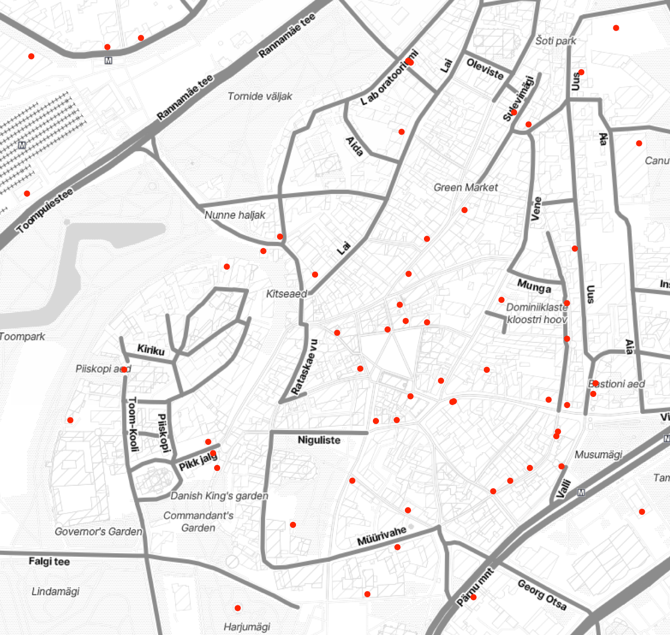
In the following example, we've extracted a set of cafes from OpenStreetMap and put them in a dataframe. All we care about for this quick visualization is the coordinates.

df = data.frame(
  lon = c(24.7408933, 24.7456935, 24.745414, 24.7455573, 24.74466, 24.7420517, 24.7406695, 24.7503795, 24.7451665, 24.7480215, 24.7465048, 24.7476525, 24.7461528, 24.745517, 24.7470942, 24.7456197, 24.7468268, 24.7433477, 24.7439016, 24.7456759, 24.7454717, 24.7492029, 24.7538602, 24.7421455, 24.7442811, 24.7499494, 24.7541156, 24.7496663, 24.7407915, 24.749436, 24.7496639, 24.7473202, 24.7500224, 24.7459907, 24.7435694, 24.737213, 24.7411354, 24.7457404, 24.744481, 24.7461543, 24.7498606, 24.7424696, 24.7478131, 24.7427942, 24.7414089, 24.7495252, 24.749662, 24.7457476, 24.7493961, 24.7483363, 24.7508932, 24.7456813, 24.7514706, 24.7467884, 24.7500806, 24.7381424, 24.7385634, 24.7482397, 24.7487323, 24.7515429, 24.7446615, 24.748973, 24.7485532, 24.7468977, 24.7454333, 24.7384107, 24.7487002, 24.7535016, 24.7389838, 24.7453955, 24.7448729, 24.7380715, 24.7503209),
  lat = c(59.4358885, 59.4383619, 59.4348787, 59.4307098, 59.4342793, 59.4386533, 59.4362213, 59.4369682, 59.4376537, 59.438031, 59.4370001, 59.4371395, 59.4388086, 59.4401727, 59.4391757, 59.4377618, 59.4367379, 59.4383531, 59.4376105, 59.4353492, 59.4379686, 59.4367582, 59.4338407, 59.43228, 59.435726, 59.4315892, 59.4293218, 59.4366903, 59.4360766, 59.4363518, 59.4375351, 59.4342403, 59.4409327, 59.4321987, 59.4333018, 59.4364968, 59.4384542, 59.4368014, 59.437154, 59.4377442, 59.4386843, 59.4388372, 59.435591, 59.4351632, 59.434102, 59.4359086, 59.4379891, 59.441055, 59.4362933, 59.4404203, 59.4414969, 59.4410772, 59.440026, 59.4367293, 59.4292313, 59.4412534, 59.4371417, 59.4357248, 59.4358888, 59.4353297, 59.4298636, 59.4320464, 59.4321256, 59.4313161, 59.4318567, 59.4440948, 59.4402673, 59.4335765, 59.4413692, 59.4364992, 59.4364868, 59.4425823, 59.4368323)
)

qmplot(lon, lat, data = df, maptype = "stamen_toner_lite", color = I("red"))

Going deeper¶

We've only shown a small part of what's possible with ggmap. You can learn more about ggmap and its capabilities on GitHub.